December 2023#
Meeting with Kaeli, Wednesday Dec. 13#
More passed electron neutrinos at lower energy#
Consider the flavor plots below (bin 1 is \(\nu_e\)).
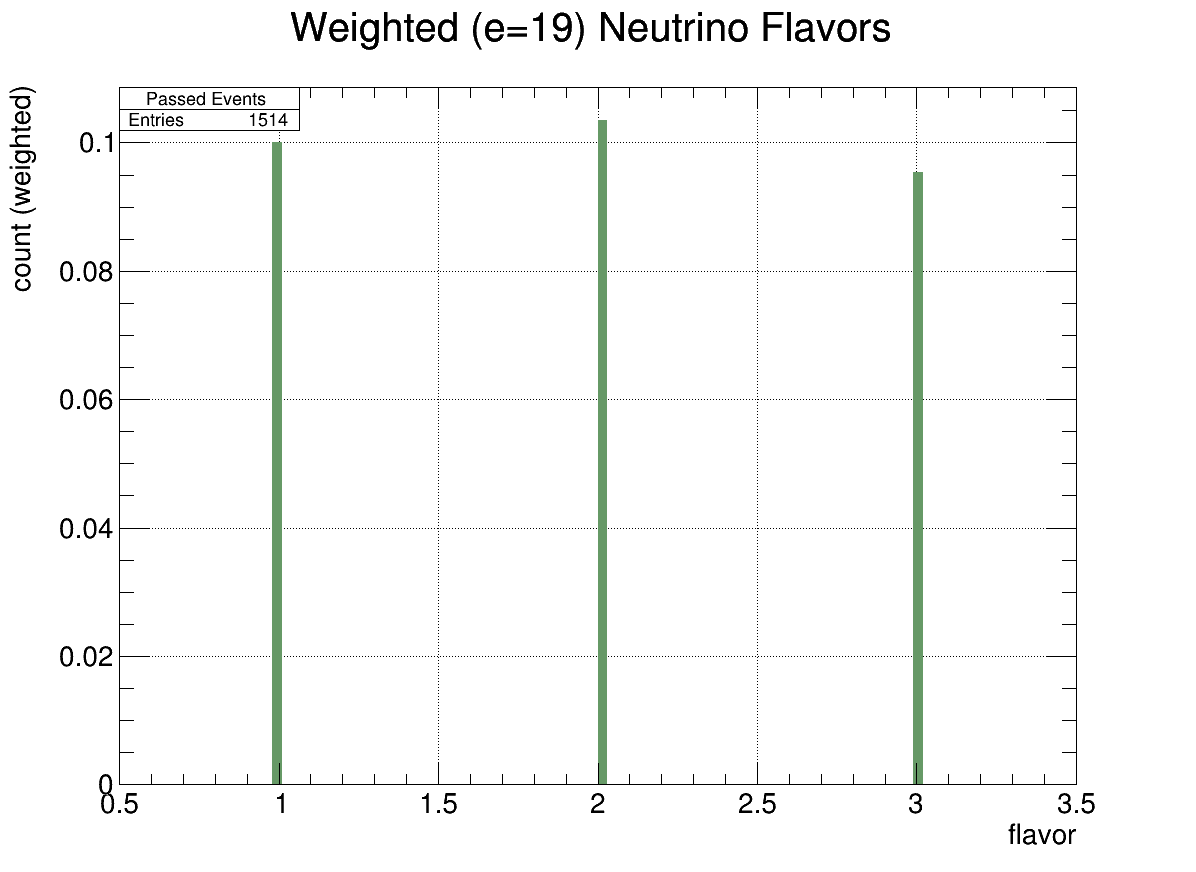
Fig. 8 Flavor Histogram (energy=19)#
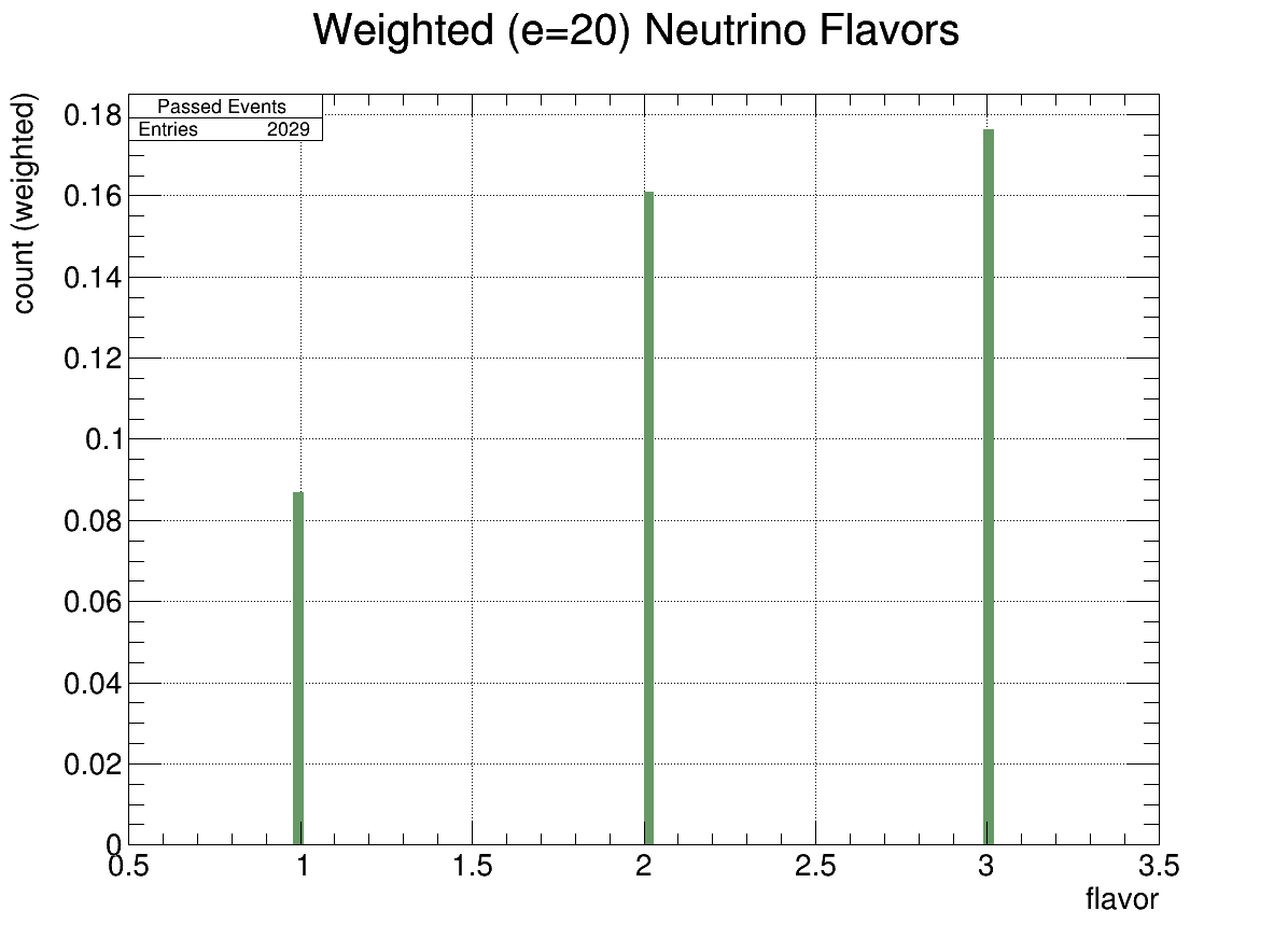
Fig. 9 Flavor Histogram (energy=20)#
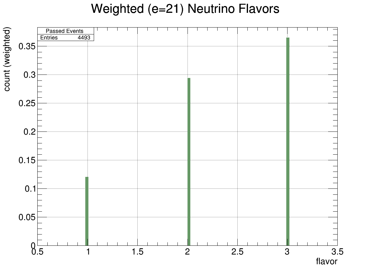
Fig. 10 Flavor Histogram (energy=21)#
We can see that at lower energies, more electron neutrinos are detected. Recall the following interactions: \( \nu_l + N \rightarrow l + X \)
\( \nu_l + N \rightarrow \nu_l + N^* \)
where \(N\) stands for nucleon (ice).If \(\nu_l\) above is an electron neutrino, then \(l=e^-\), and the electron’s energy gets immediately deposited in the ice, right where the interaction occurs and we essentially see just a bigger \(X\) (EM shower). (Think of ice as a soup of electrons, which interact with each other through EM forces)
On the other hand, if \(\nu\) above is a \(\tau\)-neutrino, then the interaction produces a \(\tau\), which does not typically deposit its energy in ice; instead, the \(\tau\) decays later as it travels in air, and we might be able to see this decay through geomagnetic emission (aka secondaries). But this is of course not the same situation as the electronic interaction, and because in this case the \(\tau\) takes away some energy, the corresponding \(X\) (EM shower) is less energetic, making it less likely to be detected.
LPM effect#
At high energies, we also see that electron neutrinos gets suppressed. This is due to the LPM effect, here are some slides
Effective Volume#
\( {\rm effective\; volume} = {\rm some\; volume} \cdot {\rm efficiency} \)
where “some volume” above for us is pretty much the entire Antarctica continent.However, the “efficiency” for us is around a fraction of a percent:
\( {\rm efficiency} = \frac{\rm weighted \; passed\; \nu}{\rm thrown\; \nu} \)In the end, PUEO’s effective volume is around 10 - 1000 km3.
Note
One can find effective volume in the source code (
report.cc?) or in the output of a simulation.
By the way, we cut some corners and define the effective area loosely as
Effective Area \(\equiv\) Effective Volume / Interaction Length
where interaction length can be found in the source code.
tasks#
Carry out the \(e=18\) run.
Read about LPM effect
For inelasticity plots, try 100 bins instead of 1000.
Make an effective volume plot
Make an effective area plot
Using awk to collect effective volumes#
I splitted the energy e=21 simulation into 100 slurm array jobs.
As an example, job No. 37 would return
37.out
.
.
.
~~~~~ Summary for electron neutrinos  ~~~~~~~~~~~~~~~
	Number simulated: 34
	Number passed (unweighted): 18
	Number passed (weighted): 0.000764247987475
	Effective volume: 6957.09761591 km^3 sr
	Effective area: 49.2280142537 km^2 sr


~~~~~ Summary for mu neutrinos  ~~~~~~~~~~~~~~~
	Number simulated: 34
	Number passed (unweighted): 12
	Number passed (weighted): 0.00709997645226
	Effective volume: 64632.462314 km^3 sr
	Effective area: 457.335508528 km^2 sr


~~~~~ Summary for tau neutrinos  ~~~~~~~~~~~~~~~
	Number simulated: 32
	Number passed (unweighted): 17
	Number passed (weighted): 0.00204211856722
	Effective volume: 19751.6638595 km^3 sr
	Effective area: 139.761613778 km^2 sr


~~~~~ Summary for all neutrinos  ~~~~~~~~~~~~~~~
	Number simulated: 100
	Number passed (unweighted): 47
	Number passed (weighted): 0.00990634300695
	Effective volume: 30660.9828112 km^3 sr
	Effective area: 216.955314155 km^2 sr

got here
finished simulation
Elapsed runtime is 1:8 minutes`
when it is completed (the output above only contains the final lines).
We can use awk to extract the information of interest; in this case, we would like to
have a script that spits out the Effective volume for all neutrinos (call it “total effective
volume”). In the example above,
this would be the line
Effective volume: 30660.9828112 km^3 sr
Below is the script I used for looping over all 100 output files contained inside an out/
directory which stores all slurm outputs.
The script returns a text file called volumes.out that contains all the 100 “total effective
volumes” for the 100 jobs of an e=21 simulation.
evol.bash
#!/bin/bash

rm volumes.out # remove if already exists.

# loop through all files in the directory "out" using a wildcard *
for file in out/*
do
     # Matching all lines that contains the word
     # "Effective volume:", get the 3rd column of the line
  awk '/Effective volume:/  {print $3}' $file  | tail -n 1 >> volumes.out
   # awk will spit out four lines. we only need the last (tail) line.

  # the following line is for debugging only. It will also display the
  # file name along with the effective volume.
  # awk '/Effective volume:/ {print FILENAME, $3}' $file  | tail -n 1
done
Below is a second version of the script above. This one utilizes GNU Awk.
evol_v2.bash
#!/bin/bash

# Note: gawk is GNU Awk, which is used because it has the "ENDFILE" check
#       which, for instance, macOS Awk does not have.
#       Note that using ENDFILE is not the same as using END

rm volumes.out

# find Effective volume line, assign it to variable a. This happens 4 times
gawk '/Effective volume:/  {a=$3}
      ENDFILE{print a}' out/*.out >> volumes.out
# However, only when we reach the end of an input file do we print out "a";
# thus, only the final match will be printed (like using >> tail -n 1)
I tested this second version on OSC. It turns out to be around 8 times faster than version one.
Presumably we would then take an average of the 100 entries of volumes.out to get the
averaged all-neutrino Effective volume. This can be done using Pandas in python:
import pandas as pd

title = ['all-neutrino effective volume']
df_21 = pd.read_csv('21_volumes.out', names=title, index_col=False)
df_20 = pd.read_csv('20_volumes.out', names=title, index_col=False)
df_19 = pd.read_csv('19_volumes.out', names=title, index_col=False)
df_18 = pd.read_csv('18_volumes.out', names=title, index_col=False)
# index_col=Flase forces pandas to not use the first column as index column and creates an
# index column starting from 0.

df = pd.DataFrame([ [18, df_18.mean()], [19, df_19.mean()],
                    [20, df_20.mean()], [21, df_21.mean()] ],
                  columns=['energy','effective volume'])


plot = df.plot.scatter(x='energy',y='effective volume',c='DarkBlue')
plot.get_figure().savefig('effective_volume.png', format='png')
The result is given in Table 15.
Energy [eV] |
Effective Volume [km\(^3\) sr] |
|---|---|
18 |
44.843654 |
19 |
2553.348809 |
20 |
13122.487126 |
21 |
24129.468761 |
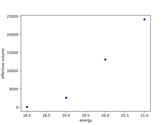
Fig. 11 An example effective volume plot#
Jan 19 Update:
Note that this is only an estimate of the effective volume.
See the January 2024 entry
for the proper way to find the average effective volume.