Using TChain to combine files

I used the following script to plot some 2 dimensional histograms.

TChain Script

void dir(){

/* ---------- setup -------------*/

  int energy=21;

  TString histogram = "Passed Events";
  std::string x_name = "x";
  std::string y_name = "y";
  TString histogram_title = "Weighted (e=" +std::to_string(energy) +") "
                            +"Neutrino XY-direction Histogram;"
                            +x_name+";"
                            +y_name;

  // initialize histogram
  TH2F * h = new TH2F(histogram, histogram_title,  
                      100, 0, 1, 100,0,1);



/* ---------- begin -------------*/

  // initialize TChain and loop through all 100 subdirectories, adding root files to chain.
  TChain chain("passTree");
  for(int i=1; i<=100; i++){

    TString file_name = 
      "../2023-11-09_nnt_100.0_energy_"+ std::to_string(energy) + "/run"
      + std::to_string(i) 
      + "/IceFinal_"
      +std::to_string(i)+"_passTree1.root";

    chain.Add(file_name); 
  }
  
  RDataFrame df(chain);


  // lambda expression that fills the histogram with entries in the chain
  auto fill_histogram = [&h] (const TVector3 &v, 
                              const double &w1, const double &w2, const double &w3){

    // total weight = path weight / (position weight * direction weight)
    double weight = w1/(w2*w3);

    h->Fill(v.X(),v.Y(),weight); 
  };


  df.Foreach(fill_histogram, {"event.neutrino.path.direction", 
                              "event.neutrino.path.weight",
                              "event.loop.positionWeight",
                              "event.loop.directionWeight"});

/* ---------- Drawing -------------*/

                       // Canvas width, height
  TCanvas * c = new TCanvas("", "", 900, 900);

        // setting the colorbar position: starts at x=1.01 and ends at x=1.02
  TPaletteAxis *palxis = new TPaletteAxis(1.01,0,1.02,1,h);
  h->GetListOfFunctions()->Add(palxis);


  gStyle->SetPalette(55);     // enables rainbow palette (up to red)
  gStyle->SetOptStat("ne");   // display only histogram name and number of entries
  h->Draw("colz");

}

Dec. 6, 2023 Update:
The script above is slightly modified (the Drawing portion) to change the size of the colorbar (compare Fig. 17 and Fig. 18). I did this following user couet’s example on the ROOT Forum.

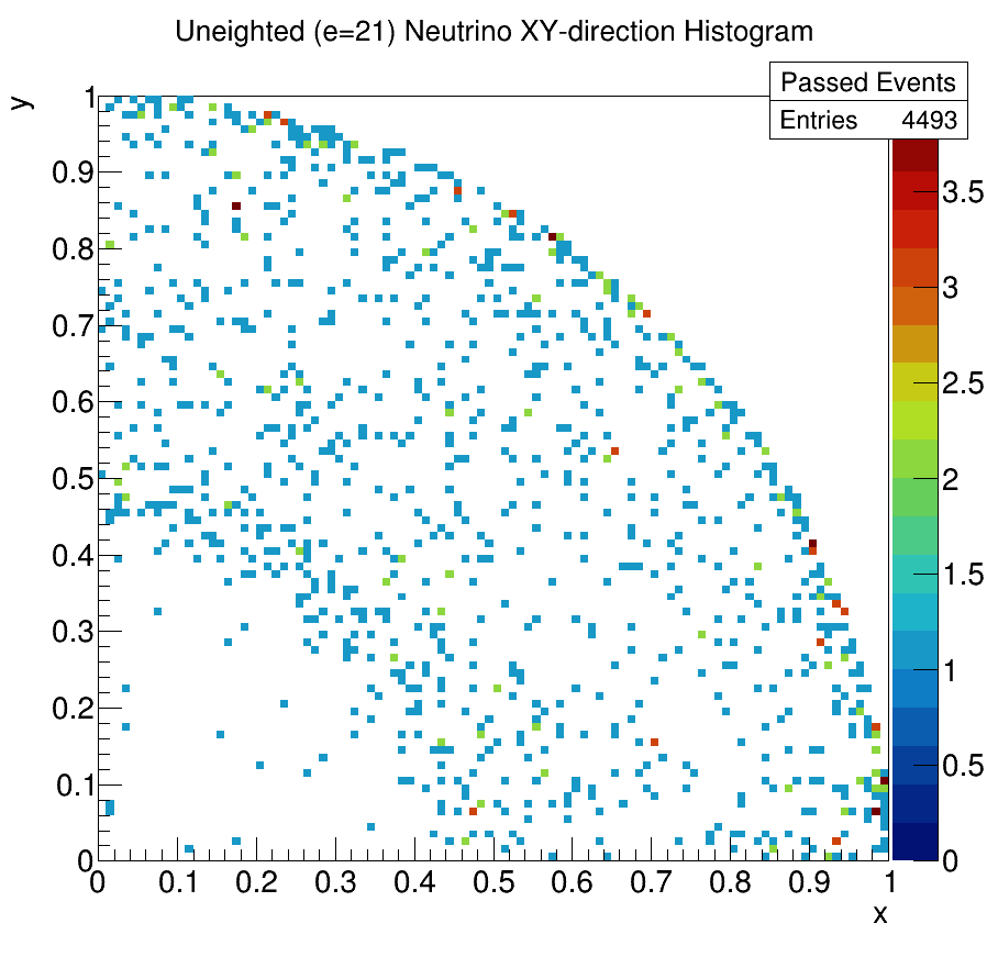
Fig. 16 Unweighted plot of direction (x and y compeonts)

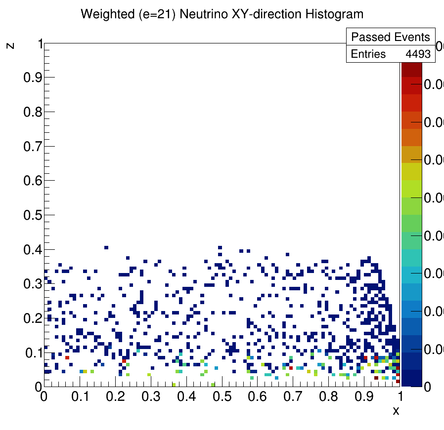
Fig. 17 Weighted plot of direction (x and z componets)

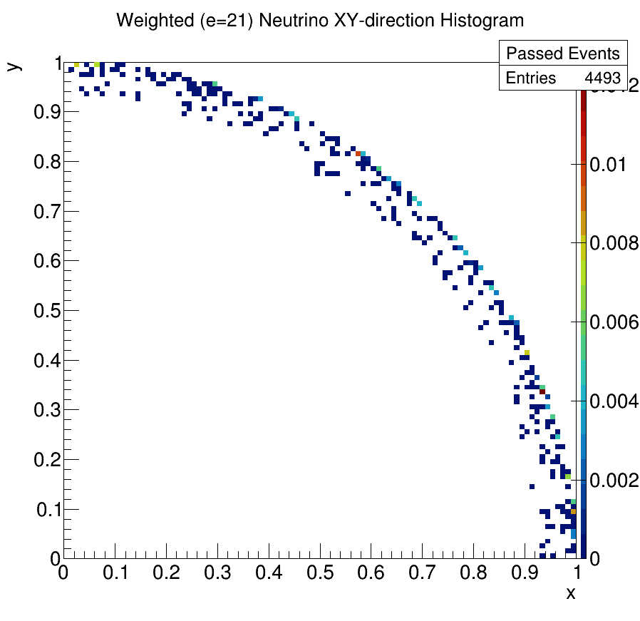
Fig. 18 Weighted plot of direction (x and y componets)