January 2024

Meeting with Kaeli, Thursday Jan. 11

logistics

• Start attending talks at least once per week, pick from below:

  • Tuesday at noon - CCAPP seminar (overhang room, PRB 4^th floor)

  • Tuesday 3:45 - Physics General Colloquium

  • Friday 11:15 - Astroparticle Lunch (Price Place)

• PUEO simulation call (Wednesday 1:00, tentative)

• individual meeting with Kaeli - Tuesday at 1:30

Effective Volume Plot

• Be sure to include units. For \(x\)-axis, use the following:
  log(energy)[eV]

• Make \(y\)-axis log scaled.

• Our systematic error is 20% (no need to include in the plot)

• statistical error normally goes like \(1/\sqrt{N}\) but is more complicated for us; will deal with this next time.

• Re-compute the effective volume!
  Instead of what I did in Dec. 2023, do the following instead.

  • Find out the (constant) total ice volume.

  • For each array-output, obtain the weighted number of passed neutrinos. Add these all up (ie. run1 passed + run2 passed + …)

  • Figure out the total number of neutrinos thrown.

  • Use the following to compute effective volume:

    \[{\rm(ice\,volume)} \cdot (4\pi) \frac{\sum{\rm number\,passed\,(weighted)}}{\sum{\rm number\,thrown }}\]

tasks

• Schedule 20 hours of research hours, put in calendar.

• Read about LPM effect

• Update the effective volume plot

• Read the GRA expectation document

Meeting with Kaeli, Tuesday Jan.16

Energy Flux

• A good resource: ask question anonymously on Slack in the #idongetit channel.
  Type "/abot #idontgetit message-content-here" to ask an anonymous question.

  Slack

  There is a question regarding single event sensitivity (SES) inside this channel. Give it a read.

• The following is in the Appendix of the paper that Kaeli will send. \(i\) denotes the \(i\)^th energy bin.

• We will plot

  \[E_i F(E_i) = \frac{n_i}{\Lambda_i \, \ln(10) {\rm d}\log_{10} E_i}\]

  where

  • \(E_i\) is the energy

  • \(n_i\) is the F-C

    Note

    0 event corresponds to an F-C of 2.44

  • \(\ln(10)\) is there for normalization

  • d\(\log_{10}E\) is the energy bin width. For example, if we plot something versus energy and the energies are \(10^{18}\), \(10^{19}\), \(10^{20}\), and \(10^{21}\), then the log (base 10) of the bin width would just be 1.

  • \(\Lambda_i\) is the exposure.

Exposure

Efficiency \(\epsilon_i\) \(\times\) Effective Area \(A_i\) \(\times\) Time \(T_i\)

Note

For simulation purposes, efficiency is 1.
Additionally, for PUEO, time is 30 days.

Effective Area

• To compute the effective area, recall that we cut corners by computing

  \[ A_{\rm eff} = \frac{V_{\rm eff}}{l_{\rm int}}\]

  where \(l_{\rm int}\) is the interaction length.

Interaction Length

How much of the Earth a neutrino penetrates before interaction occurs. (we don’t know exactly what this value is for high energy neutrinos, but we have an estimate based on extrapolation from lower energy neutrinos).

Single Event Sensitivity (SES)

TBA

TODO

Add Single Event Sensitivity (SES) glossary

tasks

• Check why my Root script is slow.

  • Make sure files are closed after opened.

  • Wed., Jan 17: Found a bug when counting the number of files for the e=18 simulation. Should be 1000 instead of 100. The end result didn’t change much on the log-log plot though.

  • I checked my TChain usage; pretty sure the memory is freed automatically the way I wrote it, so I’m not sure why the script is so slow…

• Make an effective area versus energy plot

  • Here is a table of the averaged effective volume calcuated properly as described in Effective Volume Plot.

    Table 9 Average Effective Volume

    Energy [eV]	Effective Volume [km\(^3\) sr]
    18	48.9026
    19	2784.46
    20	14310.2
    21	26313.5

    compared with Table 15, we see that there is not a huge difference. so I don’t think I made a mistake in calculating the effective volume.

  • Here is the effective area plot.

    

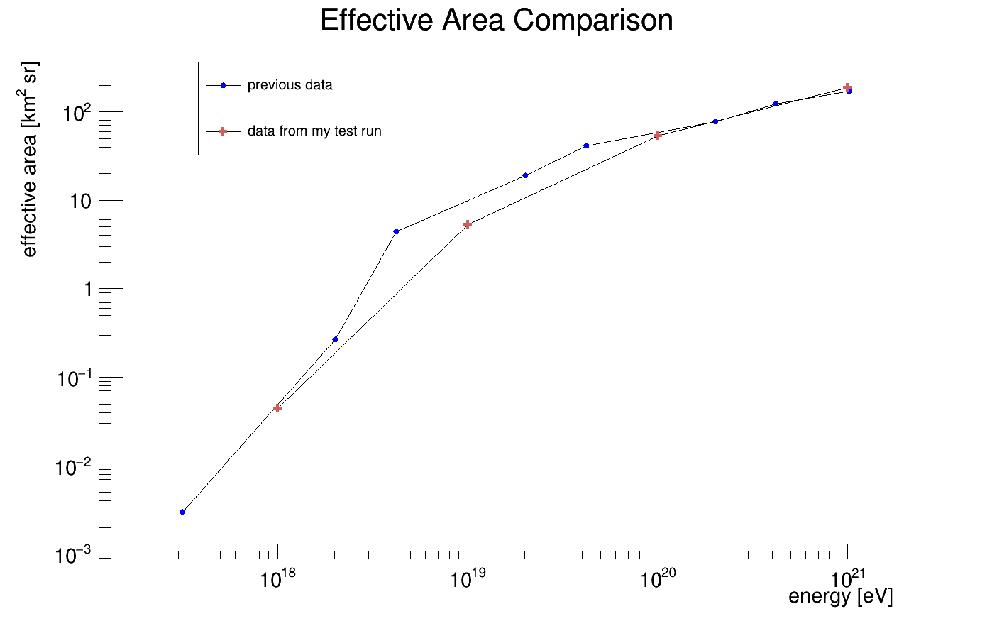
    Fig. 1 No significant difference between the previous and new effective area.

• Make a flux versus energy plot

• Read the [Upper Limit Paper]

• Read about LPM effect

Meeting with Kaeli, Tuesday Jan.23

Effective Volume Plot

• This time, include error bars.

Error-bar script from Kaeli

def AddErrors(all_weights):#the input is a numpy array of all the event weights, where each entry is an event

	#set number of bins and max/min weights
	bin_num = 10
	max_weight = np.max(all_weights)
	min_weight = np.min(all_weights)

	#set bin values for weights
	bin_values = np.linspace(min_weight,max_weight,bin_num)

	#create arrays to hold both positive and negative errors
	bin_error_p = np.zeros(bin_num)
	bin_error_m = np.zeros(bin_num)
	test_error = np.zeros(bin_num)

	#Copy poisson errors from icemc:
	poissonerror_minus=[0.-0.00, 1.-0.37, 2.-0.74, 3.-1.10, 4.-2.34, 5.-2.75, 6.-3.82, 7.-4.25, 8.-5.30, 9.-6.33, 10.-6.78, 11.-7.81, 12.-8.83, 13.-9.28, 14.-10.30, 15.-11.32, 16.-12.33, 17.-12.79, 18.-13.81, 19.-14.82, 20.-15.83]
	poissonerror_plus=[1.29-0., 2.75-1., 4.25-2., 5.30-3., 6.78-4., 7.81-5., 9.28-6., 10.30-7., 11.32-8., 12.79-9., 13.81-10., 14.82-11., 16.29-12., 17.30-13., 18.32-14., 19.32-15., 20.80-16., 21.81-17., 22.82-18., 23.82-19., 25.30-20]
	
	#histogram weights into bins
	counts, bins =np.histogram(all_weights,bins=bin_values)
	bin_centers = (bins[1:]+bins[:-1])/2.0
	bin_width = bins[1]-bins[0]

	#loop over bins:
	for i, b in enumerate(bin_centers):
		#if bin has less than 20 events, use poisson errors
		if(counts[i]<20):
			this_pp = poissonerror_plus[counts[i]]
			this_pm = poissonerror_minus[counts[i]]
		#otherwise use sqrt(N)
		else:
			this_pp = np.sqrt(counts[i])
			this_pm = np.sqrt(counts[i])
		#print('this pp pm is :',this_pp, this_pm)

		#bin error is this error times the bin width
		bin_error_p[i]=this_pp*b#*bin_width
		bin_error_m[i]=this_pm*b#*bin_width

		#this is just here to compare against what I thought icemc was doing originally (not used)
		test_error[i]=this_pp*10**(-1*(i+0.5)/bin_num*(max_weight-min_weight)+min_weight)

	#total error is then added in quadrature 
	total_error_p = np.sqrt(np.sum(bin_error_p**2))
	total_error_m = np.sqrt(np.sum(bin_error_m**2))

	#again this is just a test to compare against icemc
	total_test = np.sqrt(np.sum(test_error**2))

	return(total_error_p,total_error_m)

tasks

• Fix the bug in my effective area plot

• Do another run using the current version of PueoSim

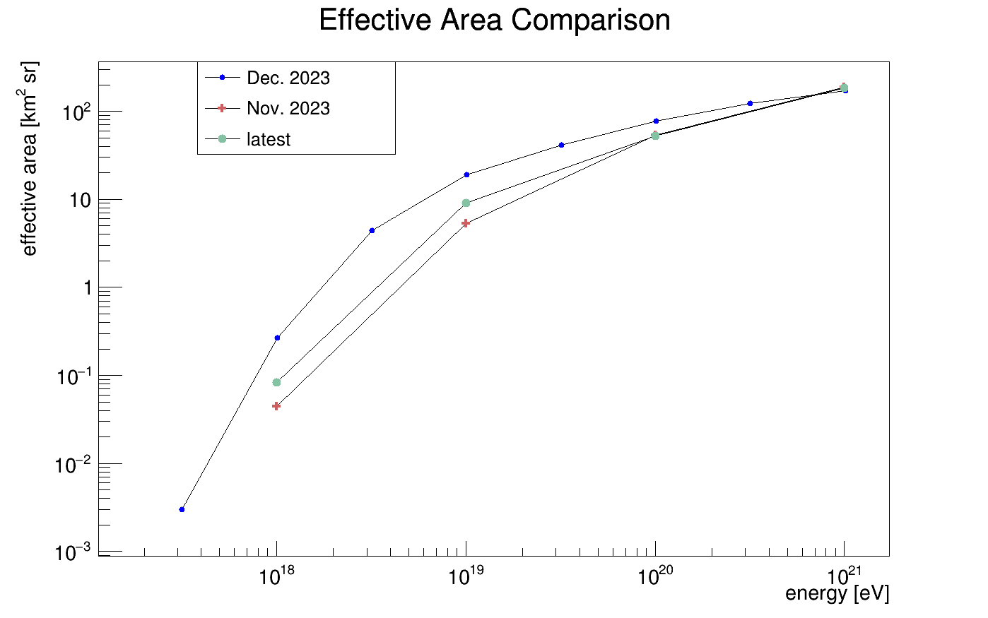
• Make a new effective area plot using all three sets of data.

  • Kaeli’s data is from Oct. 23

• Send Kaeli the flux plot

• go through the slides on reconstruction work in the database

updated effective area plot

Table 10 Number of neutrinos passed

	total number thrown	number passed	number passed (weighted)
Nov. ‘23, energy 21	10000	4493	0.779606
Nov. ‘23, energy 20	10000	2029	0.423978
Nov. ‘23, energy 19	40000	1547	0.329987
Nov. ‘23, energy 18	1000000	1324	0.144887
Jan. ‘24, energy 21	10000	4900	0.766993
Jan. ‘24, energy 20	10000	2420	0.414757
Jan. ‘24, energy 19	40000	2110	0.567759
Jan. ‘24, energy 18	1000000	1889	0.272608