June 2024#
Noise waveforms: on the ZEROSIGNAL fix.#
Here are the relevant commits that fixed the
ZEROSIGNALoption forpueoSimbefore the thermal noise update. 1,2 and 5 are critical. 5 is the actual fix, but 1 and 2 are needed for the pre-thermal-update version ofpueoSim.
On reading the flux plots.#
I have been confused by the y-axis units on these plots since forever ago. Luckily there’s a detailed explanation on StackExchange.
In case that post gets taken down, here is User Gonstasp’s reply to OP’s question.
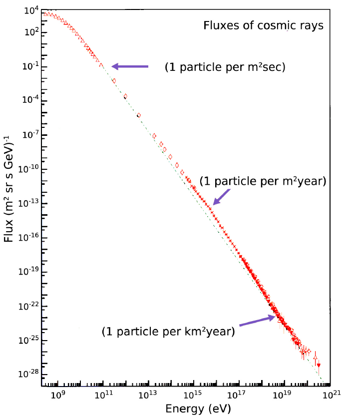
Fig. 6 Stolen plot from StackExchange.#
This graph shows the distribution of cosmic rays detected on ground (per unit of time [s], surface [\(m^2\)], energy [GeV] and solid angle [“sr”, i.e. steradian]), with respect to their energy [eV].
It is not an electromagnetic flux, but a particle flux. Cosmic rays are not photons, they are high-energy particles traveling through space (hadrons, leptons; for example protons and electrons, etc.)
You can read the graph as follows : on Earth, the incoming flux of cosmic rays with an energy
is approximately \(10^{−24}\) m\(^{−2}\) sr\(^{−1}\) s\(^{−1}\) GeV\(^{−1}\).
It means that on a 1 kilometer surface, it would require (statistically) :
to observe one cosmic ray with that energy, or approximately 6 months.
By the way, this is why the error bars are larger at the bottom-right end of the graph. These high-energy events are very rare.
…
…[Note that] given a flux of particle per second \(F\) [T\(^{-1}\)] (the dimension of \(F\) is time\(^{-1}\)), the time required to observe one particle is \(1/F\) [T] (the dimension of \(1/F\) is time)…
Actually this other post. might have a more accurate explanation.
User J. Murray’s response
The “per MeV” refers to the fact that the flux rate \(f(\theta, \phi, E)\) tells you the particle flux per unit solid angle per unit energy. That is, \(f(\theta, \phi, E) d \Omega d E\) is the particle flux (in particles per unit area per second) within a small solid angle \(d\Omega\) around \((\theta,\phi)\) and a small energy range \(dE\) around E.
If you want to find the particle flux per unit solid angle (without the energy part), then you need to interate over all energies in some range, i.e.
which is the flux of particles per unit steradian with energy between \(E_1\) and \(E_2\). It’s worth noting that when you have a histogram with energy bins \(\Delta E_i\), then the quantity being plotted is \(f(\theta,\phi,E_i) \Delta E_i\).
To obtain \(f(\theta,\phi,E)\) from a histogram, you divide the counts in each bin by the bin width. Conversely, if you have the so-called differential flux \(f(\theta,\phi,E)\) and want to know how many counts to expect in a histogram bin at some energy, you simply multiply it by the bin width.
The figure in question is this one:
The point marked “1 particle per m\(^2\)” has \(f(\theta,\phi,E) \approx 10^{-1}\) m\(^{-2}\) s\(^{-1}\) sr\(^{-1}\) GeV\(^{-1}\). If we multiply by \(4\pi\) (assuming the flux is isotropic) and a bin width of 1 GeV, then we get the right flux.
Apparently at 10\(^{11}\) eV, the bin sizes are approximately 1 GeV. The logarithmic scale suggests logarithmic binning, so at 10\(^{16}\) eV we would expect a bin size of about 10\(^5\) GeV. The plot indicates that \(f(\theta,\phi,10^{16} eV) \approx 10^{-14}\) m\(^{-2}\) s\(^{-1}\) sr\(^{-1}\) GeV\(^{-1}\), so multiplying by \(4\pi\) and 10\(^{5}\) GeV yields a flux of 0.4 particles per square meter per year, which is the right order of magnitude for the second label.
As far as interpretations go, you should take the first label as saying that about 1 particle within energy 1 GeV of \(10^{11}\) eV passes through a 1 m\(^2\) target every second. The second label tells you that about 1 particle with energy within \(10^{5}\) eV of \(10^{16}\) eV passes through a 1 m\(^2\) target every year.
An alternative way to say it is that one particle with energy within 1% of \(10^{11}\) eV passes through a 1 m\(^2\) target every second, while one particle with energy within 1% of \(10^{16}\) eV passes through a 1 m\(^2\) target every year.
And here is yet another related post
User rob’s answer
Question
I am trying to understand the X-ray emission spectrum based on medical X-ray tubes and there are several variants of the graph function given in several books as in this image:
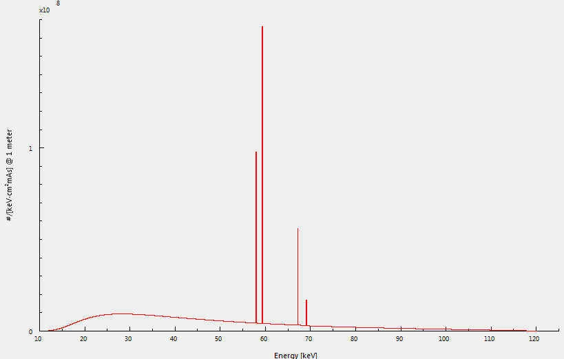
Fig. 7 Yet another stolen plot from StackExchange.#
At a specific energy (in KeV) the plot shows the number of photons emitted by an element in the units of hash/[KeV * cm\(^2\) * mAs] where Hash is the numeric value of the number of photons.
My question is regarding the units of the dependent variable of the graph function. How is there a KeV unit addedto it? Shouldn’t the number of photons have the units of hash/[cm\(^2\) * mAs] where Hash is the numeric value of the number of photons where, the photons cross an area over a particular current-time product and therefore cm\(^2\)*mAs in the denominator is understood but why a KeV term (unit) is also present?
Answer
I think the way to read you “hash” (“#”) is as a “number.”
What you’ve plotted here is a differential spectrum: the number of x-ray events observed in each energy window from \(E_i\) to \(E_i + \Delta E\) . The most common way to construct such a spectrum is to build a histogram. But in a histogram, the number of events in each bin depends on the width of the bins, \(\Delta E\). For example, if you start with a histogram that has 100 energy bins, decide it’s too noisy, and combine the odd bins with their even neighbors to produce a new histogram with 50 bins, the number of events in each bin will approximately double.
You can avoid that blurring between data and representation by displaying, rather than raw counts per bin, the counts divided by the bin width. In our 100→50 rebinning example, the number of counts in the larger bins would approximately double, but the width doubles as well: the differential spectrum doesn’t change.
Essentially, each point in your spectrum here is
where the integral of this spectrum, \(N\), is the total number of events you’d expect from the experiment. You’re not bothered by the fact that if you ran the experiment twice as long, or used a detector with twice the area, or drove twice as much current through the source, that you’d double the number of photons you find. For energy the relationship is nonlinear: the total number of events is
and what’s plotted here is the differential \(dN/dE\).
I learned this as a graduate student when I tried, unsuccessfully, to turn a plot of neutron flux versus wavelength, \(dN/d\lambda\), into a plot of neutron flux versus energy, \(dN/dE\), using the deBroglie relation \(p=\hbar/\lambda\) and the kinetic energy \(E = p^2/2m\). You can’t just re-map the points on the spectrum to the new values; you have to take into account that the denominator is different as well in order to ahve the two spectra integrate to the same \(N\).
On ANITA’s elevation angle#
\(\theta = +90^{\circ}\) corresponds to the \(-\hat{z}\) direction.
But in a way it makes sense, because if a signal is coming straight down, we will say that the signal is hitting the horizon at an elevation angle of 90 degrees.
Here is a note by Dr. Ben Strutt on the derivation of Eqn 8.3 in his thesis. In the derivation he included the definition of the elevation angle:
Ben's derivation of expected time-delay as a function of incoming signal direction (theta and phi)